Essential Statistics Homework

(Refer back to the Essential Statistics lesson).

Key Concepts

Descriptive statistics

Hypothesis testing

Normality assumptions

Cross tabulation

Logistic regression

Interpreting model summaries

The datasets we’ll be using for this assignment are both curated and hosted by the Vanderbilt Department of Biostatistics.

Stress Tests

Dobutamine is a drug that is used during echocardiograms (aka “stress tests”), which are clinical tests used to estimate heart function. The treatment causes heart rate to increase, and its effects at different dosages were measured in a study published in 1999.

We’ll be using the data behind this paper to answer the questions that follow. Use the following to read and store the data directly from the web. Feel free to load dplyr+readr or tidyverse packages and use the read_csv() function instead of base R’s read.csv().

stress <- read.csv("http://biostat.mc.vanderbilt.edu/wiki/pub/Main/DataSets/stressEcho.csv")

Note that in addition measuring dobutamine dosages during each stress test, the authors collected information on other variables including: resting heart rate, max heart rate, blood pressure, age and (most importantly) whether or not the patient experienced any cardiac event in the 12 months that followed the test.

Before answering the questions, make sure to review the data dictionary:

http://biostat.mc.vanderbilt.edu/wiki/pub/Main/DataSets/stressEcho.html

Note that the data were originally coded by the authors of the study but were then partially recoded when curated. Pay particular attention to the any.event variable (did the subject experience any cardiac event over 12 months following the stress test), which should be interpeted as 0=NO, 1=YES. The top of the data dicionary makes this clear that all event variables are recoded such that 0=no and 1=yes, which is more conventional.

What is the highest maximum heart rate double product with Dobutamine (dpmaxdo)?

## [1] 45114

What is the cutoff for the 99th percentile for the measurment above?

HINT: The quantile() function defaults to 0, 0.25, .5, .75 and 1 but can accept arbitrary threshholds. See ?quantile and look for the probs argument.

##   99% 
## 31949

Use ggplot2 to create a histogram showing the distribution of the dpmaxdo values.

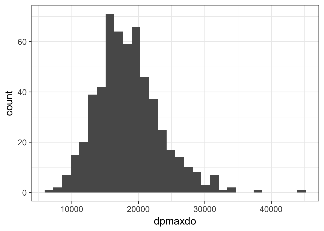
The plot above indicates that the distribution is approximately normal, with the except of a few outliers at the right tail. With the normality assumption satisfied, perform a two sample t-test to compare the mean double product max heart values between those who did or did not experience any cardiac event (any.event). Assume equal variances between these groups.

## 
##  Two Sample t-test
## 
## data:  dpmaxdo by any.event
## t = 2, df = 600, p-value = 0.04
## alternative hypothesis: true difference in means is not equal to 0
## 95 percent confidence interval:
##    60.1 2279.9
## sample estimates:
## mean in group 0 mean in group 1 
##           18736           17566

What is the p-value for this test? Make sure this is accessed from the results (using the $ operator) rather than simply re-typing the value. Feel free to extract the p-value directly from the t-test, or first use broom::tidy() to tidy the model first.

## [1] 0.0389

The smoking history column (hxofCig) is represented categorically as “heavy”, “moderate” and “non-smoker”. Create a margin table showing the total counts of individuals in each smoking history category, for all individuals who either did or did not have any cardiac event by smoking status. Next, show proportions over the row margin (what percentage of each category had any cardiac event?).

##             any.event
## hxofCig        0   1 Sum
##   heavy       98  24 122
##   moderate   115  23 138
##   non-smoker 256  42 298
##   Sum        469  89 558

##             any.event
## hxofCig          0     1
##   heavy      0.803 0.197
##   moderate   0.833 0.167
##   non-smoker 0.859 0.141

Create a mosaic plot to explore the tabulated counts visually.

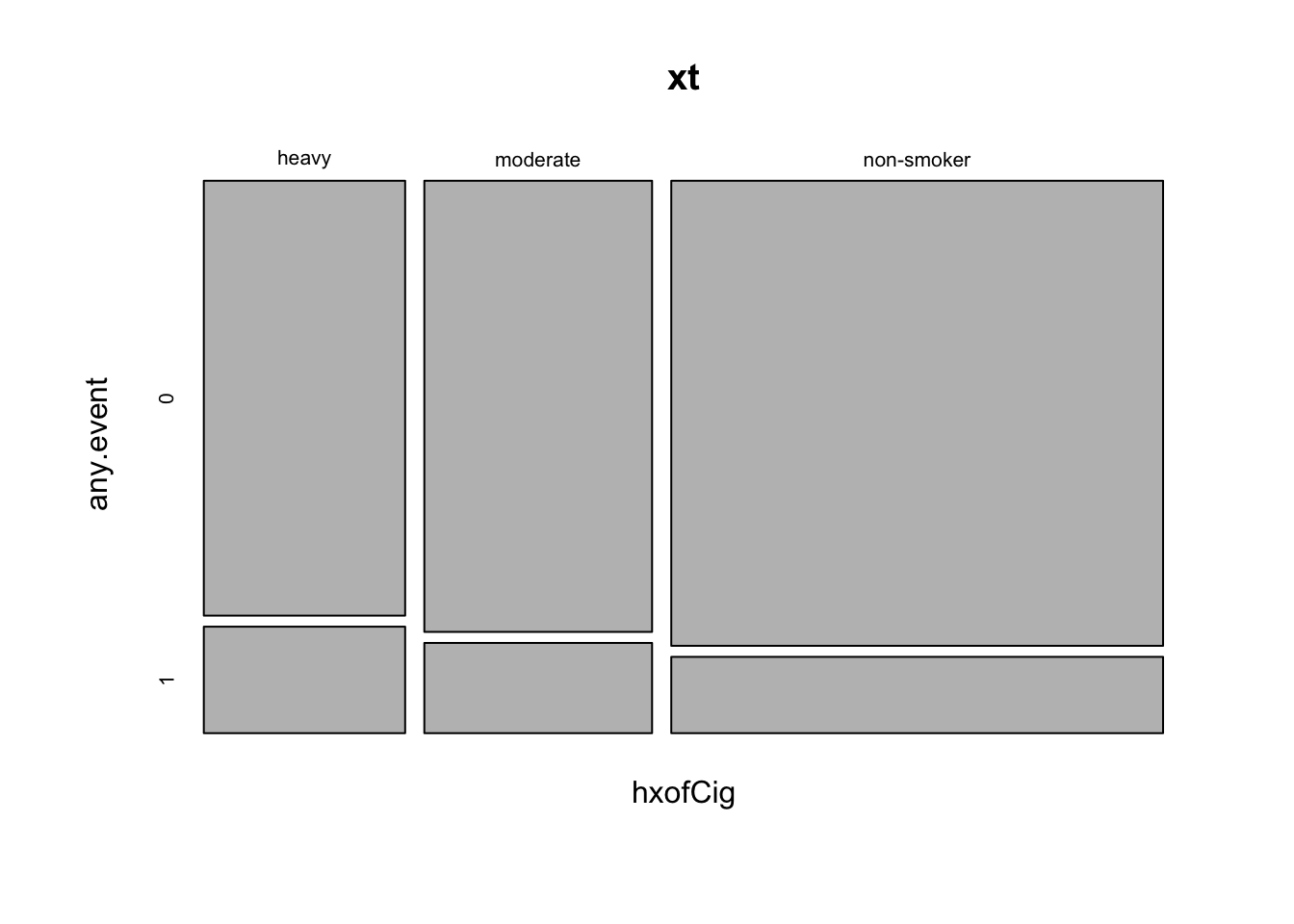
Now use a chi-squared test for the independence of smoking history and cardiac event.

## 
##  Pearson's Chi-squared test
## 
## data:  xt
## X-squared = 2, df = 2, p-value = 0.4

Load the broom package and “tidy” the model output above.

##   statistic p.value parameter                     method
## 1      2.08   0.354         2 Pearson's Chi-squared test

Muscular Dystrophy Genetics

The questions that follow are based on a data collected to examine several blood serum markers believed to be associated with genetics for a specific kind of muscular dystrophy (DMD). The data were analyzed and results reported in a 1985 paper. In particular, the authors were interested in whether a woman’s DMD carrier status (carrier) was related to the blood serum markers creatine kinase (ck), hemopexin (h), pyruvate kinase (pk) and lactate dehydrogenase (ld).

Use the following to read and store the data:

dmd <- read.csv("http://biostat.mc.vanderbilt.edu/wiki/pub/Main/DataSets/dmd.csv")

For more information on the data set see:

http://biostat.mc.vanderbilt.edu/wiki/pub/Main/DataSets/dmd.html

What is the average value for lactate dehydrogenase?

## [1] 199

The four serum markers (creatine kinase, hemopexin, pyruvate kinase and lactate dehydrogenase) are all predictors of interest in this case. Use ggplot2 to create histograms to assess the normality of the distribution for each of these variables.

HINT: The plot below uses gather() from tidyr to transform the data so all histograms can be rendered in a single “facet wrapped” plot. Feel free to give this a shot or create separate histograms for each variable. Either method is acceptable.

## Warning: Removed 15 rows containing non-finite values (stat_bin).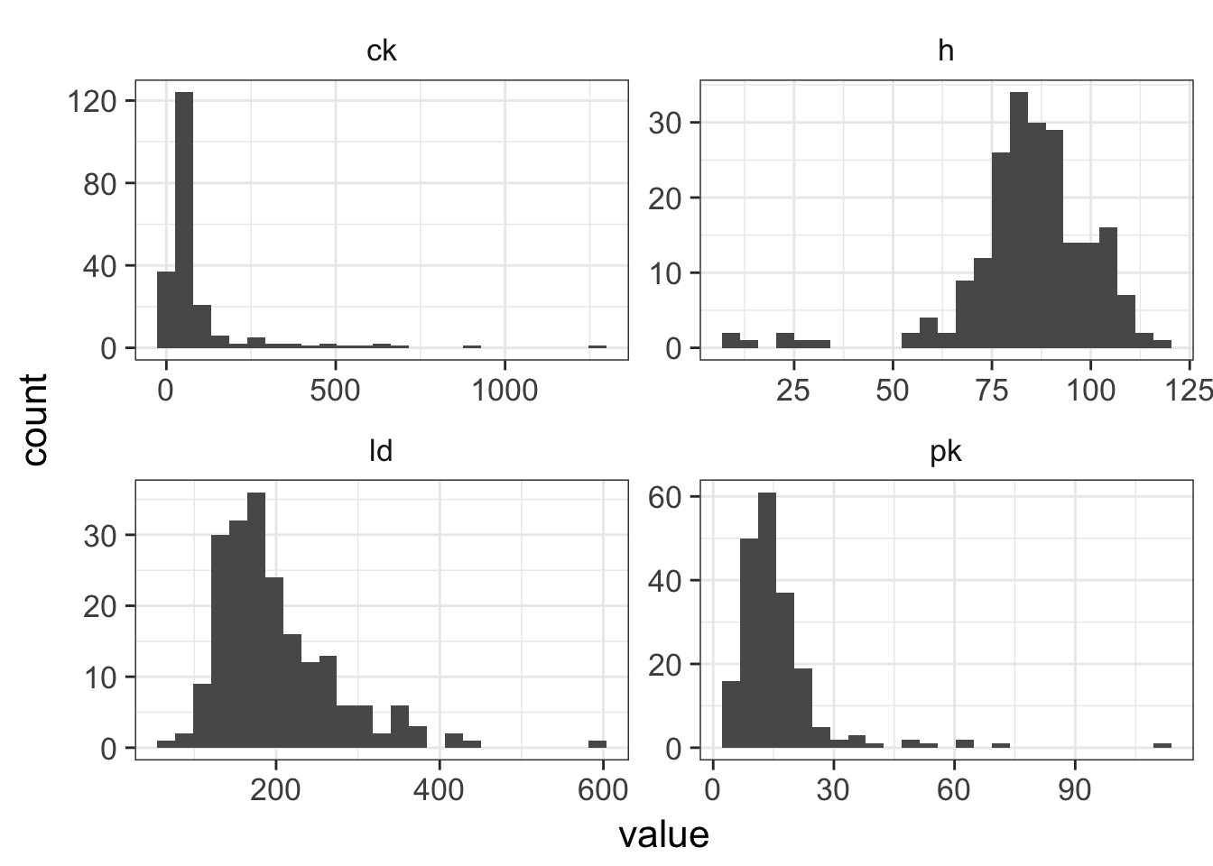

All of these columns have outliers and are (at least slightly) skewed. But ck seems to require the most attention. Try using a log transformation on that column and create another histogram.

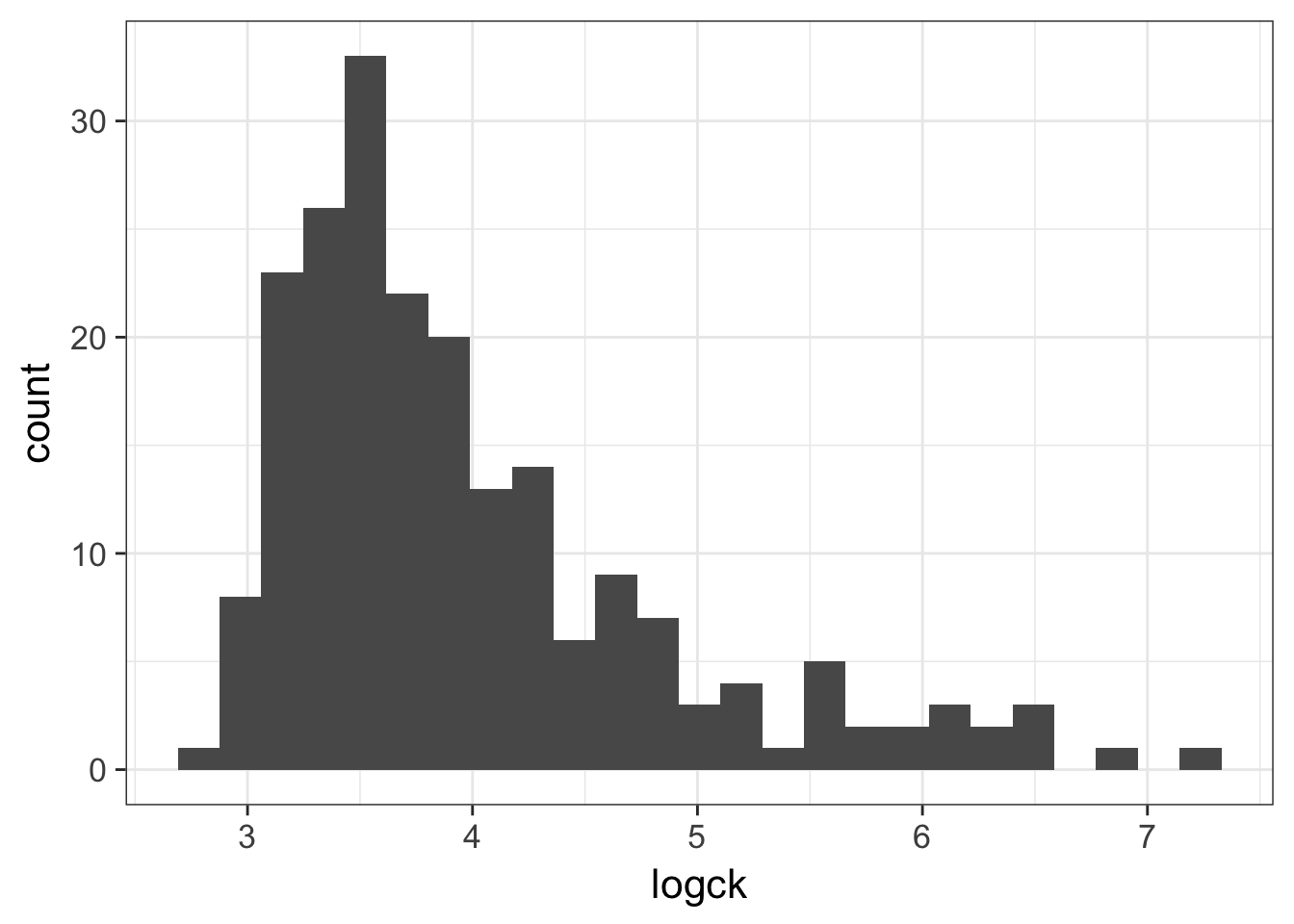
Even when transformed, the cytokine kinase is a little skewed. Assuming we can tolerate this, let’s try fitting a binary logistic regression model that predicts the mother’s status as carrier based on the values of the four blood serum markers. Don’t forget to use the log version of ck, and to use summary() on the model object to view the coefficients.

## 
## Call:
## glm(formula = carrier ~ log(ck) + h + pk + ld, family = "binomial", 
##     data = dmd)
## 
## Deviance Residuals: 
##     Min       1Q   Median       3Q      Max  
## -2.3512  -0.4151  -0.1539   0.0829   2.4006  
## 
## Coefficients:
##              Estimate Std. Error z value Pr(>|z|)    
## (Intercept) -25.95891    4.28709   -6.06  1.4e-09 ***
## log(ck)       2.86251    0.65632    4.36  1.3e-05 ***
## h             0.11280    0.02825    3.99  6.5e-05 ***
## pk            0.10321    0.04378    2.36    0.018 *  
## ld            0.01284    0.00526    2.44    0.015 *  
## ---
## Signif. codes:  0 '***' 0.001 '**' 0.01 '*' 0.05 '.' 0.1 ' ' 1
## 
## (Dispersion parameter for binomial family taken to be 1)
## 
##     Null deviance: 250.077  on 193  degrees of freedom
## Residual deviance:  99.005  on 189  degrees of freedom
##   (15 observations deleted due to missingness)
## AIC: 109
## 
## Number of Fisher Scoring iterations: 7

The coefficient (estimate) for each explanatory variable gives us the log of the odds ratio. Exponentiate the estimates to make them more interpretable (i.e. the odds ratio for each 1-unit increase in the predictor variable).

## (Intercept)     log(ck)           h          pk          ld 
##        0.00       17.51        1.12        1.11        1.01